Coherent Multiplex
A real-time signal analysis and visualization platform that combines advanced signal processing with graph-network based interfaces. The app procedurally generates synthetic signals, analyzes their relationships using multiple metrics, and presents the results visually.
Core Functionality
- Signal Generation & Processing: Generates synthetic signals (labeled A-H) with multiple sine wave components, random frequencies, phases, and amplitudes. All features are procedurally generated and include dynamic envelope shaping, time-varying noise, random coherent relationships (10% pairs), and signal dropouts. Uses the Fastest Fourier Transform in the West C subroutine for high-performance FFT computation.
- Advanced Analysis: Wavelet coherence analysis (powered by fCWT), phase relationships, and cosine similarity for frequency spectra. Identifies related signals and valid analysis regions.
- Real-time Streaming: Python and C backends stream live data via SSE, updating every second with new signal, FFT, and coherence results. Maintains a 256-point rolling buffer.
Visualization Features
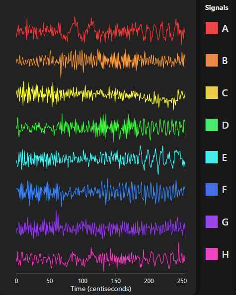
- Time Domain: Real-time visual of signals with color-coded traces.
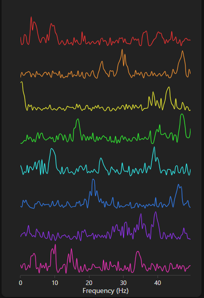
- Frequency Domain: Live frequency magnitude spectra for each signal.
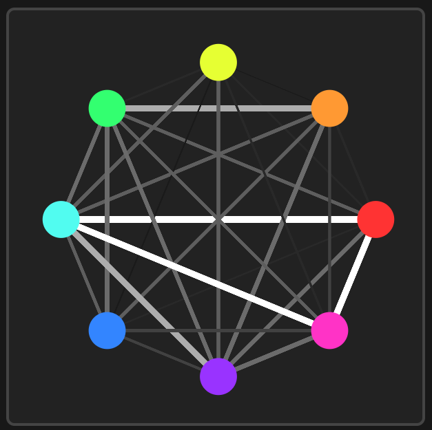
- Network Graph: Javascript-powered interactive graph showing signal relationships with dynamic edges.
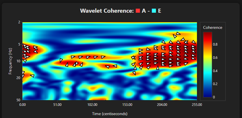
- Coherence Heatmap: Scientific visualization of wavelet coherence with phase arrows to show lead-lag.
- Similarity Panel: Live display of cosine similarity metrics between all signal pairs.
Coherent Multiplex: Real-Time Signal Coherence Analysis and Feature Extraction Platform
Abstract
The Coherent Multiplex is a real-time signal analysis and visualization platform designed to identify and monitor coherent relationships among multiple time series signals. By combining fast Fourier analysis, wavelet coherence, and interactive graph representations, the Multiplex enables efficient exploration of dynamic interactions in live signals. This whitepaper introduces the system architecture, core methodology, current prototyping efforts, and potential applications in research, trading, and live monitoring. Possibilities and goals for future directions with the Multiplex are also discussed.
Introduction
Understanding and employing wavelet coherence between signals is becoming increasingly popular in fields like neuroscience, finance, geophysics, and communications, where uncovering relationships between signals can reveal underlying mechanisms and patterns. Conventional approaches to coherence analysis are limited to high-level programming languages, run outdated transforms, and are incapable of handling high-volumes or real-time data streams efficiently. The Coherent Multiplex overcomes these challenges by offering a rapid and scalable solution for live coherence tracking, allowing users to explore frequency- and time-dependent interactions with greater speed and precision.
By leveraging advanced algorithms and optimized computing frameworks in the Fastest Fourier Transform in the West (FFTW) and the Fast Continuous Wavelet Transform (FCWT), the Multiplex significantly reduces the processing time required for coherence analysis, making it suitable for real-time and large-scale applications. This innovation, combined with the living multilayered network architecture, will enable researchers and industry professionals to efficiently monitor and investigate dynamic signal relationships as they evolve, supporting new opportunities in data-driven decision making and responsive system design across diverse scientific and industrial domains.
System Overview
- Signal Ingestion: Flexible APIs and device connections for diverse data sources.
- Real-Time Spectral Transform Compute: Fast Fourier transforms for immediate spectral insight.
- Multilayered Graph Network: Nodes represent signals, edges represent coherence/similarity.
- Pairwise Cosine Similarity Analysis: Quantifies spectral alignment between signals.
- Selective Wavelet Coherence: Time-frequency resolution of dynamic interactions using CWT.
- Interactive Dashboard: Time-domain plots, FFT spectra, network graphs, and heatmaps with live updates.
Technical Outline
Incoming Data
A live signal can be represented as a real-valued function of time:
where $x(t)$ is defined only up to the present moment $t_0$:
A continuous-time signal $x(t)$ sampled at a frequency $f_s$ (in Hz) becomes:
where $f_s$ is the sampling frequency (samples per second), and $n$ is the discrete time index. For the real-time processing employed by the Multiplex, a finite-length buffer is defined:
where $N$ is the window size.
Multiple signals are indexed by $i \in\{1, \dotsc, M\}$, each with its own discrete-time sequence and buffer $X_i[n]$. By aligning our signals in an M-dimensional vector, the full datastream is represented in the $N \times M$ matrix D:
Frequency Domain
To analyze the spectral properties of each signal, a discrete Fourier transform (DFT) is applied row-wise to the data matrix $D$. For a discrete-time signal $X_i[n]$, its DFT over the window of size $N$ is defined as:
where $f_i[k]$ represents the complex frequency component at bin $k$, and i is the imaginary unit. This transform yields a frequency-domain representation of each signal, capturing its harmonic content within the sliding buffer. The entire frequency-domain data across all $M$ signals is represented by the matrix $F \in \mathbb{C}^{M \times N}$, where:
Each row corresponds to a signal's frequency spectrum, and each column represents a particular frequency bin across all signals.
As long as the incoming signal data is real-valued, the Fourier values will exhibit Hermitian symmetry, meaning:
where $\overline{X[\cdot]}$ denotes the complex conjugate. This symmetry implies that the frequency components for positive frequencies uniquely determine those for negative frequencies, allowing the Fourier transform of a real signal to be fully represented by the first $L = \left\lfloor \frac{N}{2} \right\rfloor + 1$ frequency bins (including the zero-frequency and, if $N$ is even, the Nyquist frequency). Exploiting this property, matrix $F$ can be safely reduced to $F_r \in \mathbb{C}^{M \times L}$.
Cosine Similarity
To identify signal pairs with similar spectral profiles, Coherent Multiplex computes the pairwise cosine similarity between rows of the reduced frequency matrix $F_r \in \mathbb{C}^{M}$. Given two complex-valued frequency vectors $f_i$ and $f_j$, their cosine similarity is defined as:
where $\langle f_i, f_j \rangle$ denotes the complex inner product:
and $\|f_i\|$ is the Euclidean norm:
This metric yields a real-valued similarity score between 0 and 1, where 1 indicates perfect spectral alignment. The resulting vector of similarities is defined as:
where $p = \binom{M}{2}$ is the number of unique unordered signal pairs.
Exploratory Network
The similarity vector $S$ is used to construct a fully connected graph to represent the relationships among the $M$ signals. Each signal corresponds to a node in the network, and every pair of nodes $(i, j)$ is connected by an edge weighted by the cosine similarity score $s(i,j)$.
Formally, the network $G = (V, E, W)$ is defined as follows:
- $V = \{1, 2, \dotsc, M\}$ is the set of nodes, each representing a signal.
- $E = \{(i, j) \mid i, j \in V, i \neq j\}$ is the set of edges connecting every distinct pair of nodes.
- $W: E \to [0,1]$ assigns weights to edges, where $W(i,j) = s(i,j)$ is the cosine similarity between signals $i$ and $j$.
This weighted network layer encodes the spectral similarity structure among signals, enabling subsequent layer construction.
Wavelet Coherence
To uncover time-localized, frequency-specific relationships between signals, the Coherent Multiplex contains a second, sparse layer where the edges represent wavelet coherence.
To compute coherence, wavelet transform arrays must be constructed for participating nodes. Given a signal $x$, the wavelet transform is computed as:
where $\psi$ is a complex-valued mother wavelet, $s$ is the scale parameter (related to frequency), $t$ is the time index, and $\psi^*$ denotes the complex conjugate.
The wavelet coherence between signals $x_i$ and $x_j$ is then defined as:
where $S(\cdot)$ is a smoothing operator in both time and scale, and the result satisfies $0 \leq C_{ij}(t, s) \leq 1$. Edges of this layer are constructed and decay based on the corresponding edge's power from the previous exploratory layer.
Prototyping
Signal Simulation
Incoming data is procedurally generated to show signals that come in and out of covariance. 8 input signals are synthesized as linear combinations of sine waves with randomized amplitudes, frequencies, and phases. This emulates the complex, non-stationary behavior of real-world signals. Coherence is artificially introduced between selected pairs by sharing frequency components or phase structure at randomized intervals.
Buffering and FFT Analysis
For each update, the FFT is computed using a fast backend with pre-aligned reusable memory buffers. This implementation imports the FFTW C subroutine, which will enable scaling up. The magnitude spectra of the FFT results are extracted and used to compute pairwise cosine similarity. This provides a first-pass screening of potentially coherent signal pairs based on their frequency-domain peaks.
Graph Construction
A fully connected network is made to represent the 8 signals as nodes, and the edges between nodes are weighted by the cosine similarity between the corresponding signals' frequency-domain vectors. This network serves as the first layer of analysis, allowing visualization of potential coherence relationships and identification of candidate pairs for further analysis.
Wavelet Coherence
For deeper analysis in time and frequency relationships, wavelet coherence is selectively computed between the pair exhibiting the highest similarity at each update. Transform arrays are efficiently computed via the FCWT algorithm for each signal, and coherence is evaluated in the time-frequency domain. Visualizations in this implementation include phase arrows indicating lead/lag relationships but ignore the cone of influence, which masks regions that are unreliable.
Applications
Though originally developed for examining multi-decade correlations between the El Niño-Southern Oscillation and monsoon activity in South Asia, wavelet coherence has been applied broadly across numerous domains. Applications with interest in these time-frequency relationships include economics, neuroscience, mechanical and electrical engineering and bio-medical signals.
In economics, wavelet coherence analysis is widely used to investigate the dynamic relationships between financial time series, such as stock indices, exchange rates, and macroeconomic indicators. By allowing researchers to examine correlations at different time scales and periods, wavelet coherence has enabled the identification of transient co-movements and structural changes in markets that may not be visible through traditional methods.
In neuroscience, wavelet coherence provides a powerful tool for exploring the synchronization and functional connectivity between different regions of the brain. For example, it has been applied to electroencephalogram (EEG) and magnetoencephalogram (MEG) data to detect time-varying patterns of coherence between neural signals, helping to identify underlying mechanisms for cognitive processes, brain disorders, and responses to stimuli. Coherence is also used to examine correlations across physiological processes such as heart rate and respiration, enabling detection of abnormal patterns and assessment of disease impacts.
In all of these fields, coherence is studied by first selecting signals of interest from a large pool. EEG for research will regularly employ 128 - 512 nodes in high-density mappings. The NYSE National platform continuously updates the prices of over 8000 listed securities. Traditional coherence implementations would never be considered as methods of extraction for the entire corpus. The Coherent Multiplex is capable of executing these computations at scale, and is highly optimized for performance. The model can be tuned to accommodate hardware, and the most recent prototype is hosted smoothly on a basic dual-core, 3.5 GB RAM cloud platform.
Future Work
The Multiplex architecture described in this whitepaper can be summarized as heuristics for distinguishing signal pairings worthy of deeper analysis at a given time. The "heuristics" and "deeper analysis" in this case refer specifically to FFT, cosine similarity, and wavelet coherence, though this can be appended or substituted depending on the goal. If scale-independency is not necessary for the object of study, the cross-wavelet transform can be substituted in for coherence. A different metric could be used to determine the edge powers in the graph, supposing the spectral content is not the object of interest in the incoming signals.
Additional layers, both sequential and non-sequential, will be appended to the multiplex. Wavelet coherence can be calculated alongside traditional metrics like macro trends for high-powered edges in the graph, giving a more complete extraction of possible features. Additionally, subsequent layers with trained convolution neural networks will be added for automated analysis and description of the coherence readings.
References
- Frigo, M. & Johnson, S. G. (2005). The Design and Implementation of FFTW3. Proceedings of the IEEE, 93(2), 216–231.
- Grinsted, A., Moore, J. C., & Jevrejeva, S. (2004). Application of the cross wavelet transform and wavelet coherence to geophysical time series. Nonlinear Processes in Geophysics, 11(5/6), 561–566.
- Torrence, C. & Compo, G. P. (1998). A Practical Guide to Wavelet Analysis. Bulletin of the American Meteorological Society, 79(1), 61–78.
- Arts, L.P.A., van den Broek, E.L. (2022). The fast continuous wavelet transformation (fCWT) for real-time, high-quality, noise-resistant time–frequency analysis. Nat Comput Sci 2, 47–58.